Week 2: Signals and Basis Functions: Composition and Decomposition
These notes are inspired by slides made by T.A Aya Fawzy, 2015.
Basic Signals
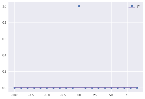
Impulse Function (Dirac)
\[\delta(x) = \left\{ \begin{array}{ll} \infty & \quad x = 0 \\ 0 & \quad x \neq 0 \end{array} \right.\]def impulse(x):
return 1 * (x == 0)
ts = np.arange(-10,10,1)
impulse_sig = impulse( ts )
stem( ts, impulse_sig )
Plotting Signals
def plot( t , y ):
    fig = plt.figure()
    ax = fig.gca()
    ax.set_ylim((-2, 2))
    ax.grid(True)

    plt.plot( t , y )

def plot2( t , y1 , y2 ):
    fig = plt.figure()
    ax = fig.gca()
    ax.set_ylim((-5, 5))
    ax.grid(True)

    plt.plot( t , y1 , 'C1', label='C1' )
    plt.plot( t , y2 , 'C2', label='C2')
    plt.legend()

def stem( t , y1 ):

    markerline, stemlines, baseline = plt.stem(t, y1, markerfmt='o', label='y2')
    plt.setp(stemlines, 'color', plt.getp(markerline,'color'))
    plt.setp(stemlines, 'linestyle', 'dotted')

    plt.legend()
    plt.show()


def stem2( t , y1 , y2 ):
    markerline, stemlines, baseline = plt.stem(t, y1, markerfmt='o', label='y1')
    plt.setp(stemlines, 'color', plt.getp(markerline,'color'))
    plt.setp(stemlines, 'linestyle', 'dotted')

    markerline, stemlines, baseline = plt.stem(t, y2, markerfmt='o', label='y2')
    plt.setp(stemlines, 'color', plt.getp(markerline,'color'))
    plt.setp(stemlines, 'linestyle', 'dotted')

    plt.legend()
    plt.show()
Unit Step Function (Heaviside)
\[\mathcal{H(x)} = \left\{ \begin{array}{ll} 0 & \quad x \leq 0 \\ 1 & \quad x > 0 \end{array} \right.\]def step(x):
return 1 * (x > 0)
ts = np.arange(-10,10,0.01)
step_sig = step( ts )
plot( ts , step_sig )

Sinusoids
def periodic_signal( freq , amp , func ):
    ts = np.arange( 0 , 0.3 , 1 / (50 * freq) )
    phases = 2 * np.pi * freq * ts
    ys = amp * func( phases )
    return ts , ys

def sin_signal( freq , amp ):
    return periodic_signal( freq, amp, np.sin )

def cos_signal( freq , amp ):
    return periodic_signal( freq, amp, np.cos )
Cosine and Sine
fig = plt.figure()
ts  ,cos_sig = cos_signal( 10 , 1 )
plot( ts, cos_sig )

fig = plt.figure()
ts  ,sin_sig = sin_signal( 10 , 1 )
plot( ts, sin_sig )
Basic Operations
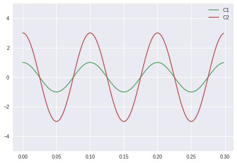
Scaling
ts  ,cos_sig = cos_signal( 10 , 1 )
cos_sig_scaled = 3 * cos_sig
plot2( ts, cos_sig , cos_sig_scaled )
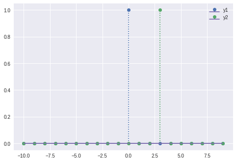
Time Shifting
ts = np.arange(-10,10,1)
impulse_sig = impulse( ts )
impulse_sig_shifted = impulse( ts - 3 )
stem2( ts, impulse_sig , impulse_sig_shifted)
Time Reversal (Mirroring)
ts = np.arange(-10,10,0.01)
step_sig = step( -ts )
plot( ts , step_sig )

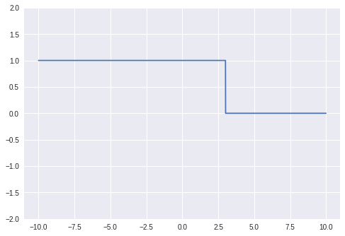
Time Reversal + Shifting
ts = np.arange(-10,10,0.01)
step_sig = step( -(ts-3))
plot( ts , step_sig )
DSP General Scheme

Sampling: Motivation
- Analog signal contains an infinite number of points.
-
The infinite points cannot be processed by computer, since they require:
- Infinite amount of memory.
- Infinite amount of processing power for computations.
- Sampling can solve such a problem by taking samples at a fixed time interval or sampling period T.
Sampling: Definition

Uniform Sampling
Task1 Requirement 1: Sampling Sinusoids and Exponential
Plot several sinusoids and exponential signals from nature, then show the sampled version of these signals.
- Python Implementation.
- Plotly, or Plotly-Dash is a plus.
- Porting your implementation on the cloud (github) is a plus.
Task1 Requirement 2: Listening to Sinusoids
Generate a sound signal composed from different sinusoids, and other from mixture of sinusoids and exponentials.
Recommended watching and reading:
Effect of Phase Shift
What is the effect of adding two sinusoids with different phase shift?
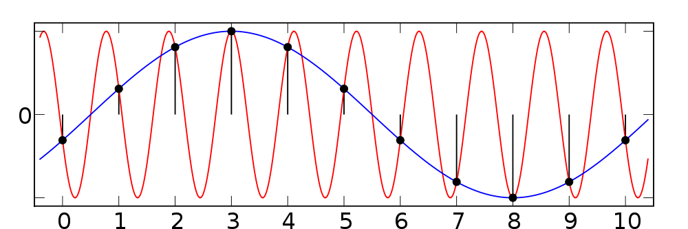
Aliasing
Nyquist Criterion
Convolution: Definition
- Convolution plays an important role in digital filtering.
- Convolution notation \(y(n) = x(n) * h(n)\)
- Convolution formula \(y(n) = \sum_{n=-\infty}^{\infty} x(n) h( n - k )\)
From Wikipedia

Textbook Problems
Example
Let \(f = \big[1,4,2,5 \big]\), \(g = \big[3, 4, 1\big]\) Estimate the convolution version of \(c = f * g\)
Solution:
Task 2: Migrating your Latest Task to Plotly
Migrate a simplified version of signal viewer task of last week, from MATLAB to Python. Also, integrate task 1 of this week into your GUI.
Deadline Wednesday of 28 Fubruary.
Code Snippets
git clone https://github.com/sbme-tutorials/sbe309-week2-demo.git