Assignment 2: Spatial domain filters, Images in frequency domain
Objectives
- 2D Convolution.
- Image Histograms.
- Histogram Equalization.
- 2D Fourier Transform.
- Image Gradients.
Prerequisites (Before you start)
- Read Section 3 Notes.
- Read Section 4 Notes.
Deadline
Tuesday 13/3/2018 12:00 PM.
Required
Each individual student is required to submit the solution of assignment problems. You can submit it as a hard-copy or scan it and send by mail providing this title (CV2018-Assignment2-[YOUR_NAME])
Problem 1
Consider the following small image:
\[\begin{bmatrix} 1 & 2 & 3 & 4 & 5 & 6 & 7\\ 1 & 2 & 3 & 4 & 5 & 6 & 7\\ 1 & 2 & 3 & 4 & 5 & 6 & 7\\ 1 & 2 & 3 & 94 & 5 & 6 & 7\\ 1 & 2 & 3 & 4 & 5 & 6 & 7\\ 1 & 2 & 3 & 4 & 5 & 6 & 7\\ 1 & 2 & 3 & 4 & 5 & 6 & 7\\ \end{bmatrix}\]a) Calculate the image that results from convolution with the following kernel:
\[\begin{bmatrix} 1 & 1 & 1\\ 1 & 1 & 1\\ 1 & 1 & 1\\ \end{bmatrix}\]Just provide the result for the central 5 by 5 part of the image.
b) Calculate the image that results from applying a 3 × 3 median filter
Just provide the result for the central 5 by 5 part of the image.
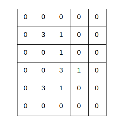
Problem 2
Calculate the following
a) The output of 3x3 mean filter
b) The output of 3x3 laplacian filter
\[\begin{bmatrix} 0 & 1 & 0\\ 1 & -4 & 1\\ 0 & 1 & 0\\ \end{bmatrix}\]c) The Histogram of the image
d) The output of histogram equalization. Show cumulative curve
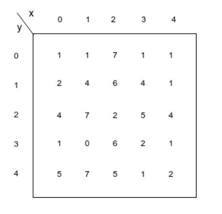
Problem 3
Let \(F(u,v)\) is the 2D DFT of the image \(f(x,y)\)
Calculate :
a) \(F(0,0)\)
b) \(F(0,1)\)
c) \(F(1,1)\)
Problem 4
The gradient of a two-dimensional function is a vector-valued derivative. The x component of the gradient is defined by
\[\begin{equation} \frac{\partial f(x,y)}{ \partial x} \end{equation}\]Consider the following three discrete approximations to the x component of the gradient of an image f. For each case, determine a convolution kernel that produces an image containing the given approximation of the x component of the gradient.
a) \(f(n_1 + 1, n_2) − f(n_1, n_2)\)
b) \(f(n_1, n_2) − f(n_1 − 1, n_2)\)
c) \(5 ∗ [f(n_1 + 1, n_2) − f(n_1 − 1, n_2)]\)
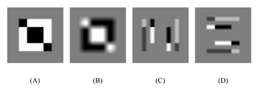
Problem 5
Consider the 48×48 input image in shown figure.

Identify which of the output images in result from applying \(h_1[n_1, n_2]\) and \(h_2[n_1, n_2]\) to the original input image, where:
\[h_1[n_1, n_2] = \begin{bmatrix} 0 & \frac{-1}{3} & 0\\ 0 & \frac{-1}{6} & 0\\ 0 & 0 & 0\\ 0 & \frac{1}{6} & 0\\ 0 & \frac{1}{3} & 0\\ \end{bmatrix}\]and
\[h_2[n_1, n_2] = \begin{bmatrix} \frac{1}{25} & \frac{1}{25} & \frac{1}{25} & \frac{1}{25} & \frac{1}{25} \\ \frac{1}{25} & \frac{1}{25} & \frac{1}{25} & \frac{1}{25} & \frac{1}{25} \\ \frac{1}{25} & \frac{1}{25} & \frac{1}{25} & \frac{1}{25} & \frac{1}{25} \\ \frac{1}{25} & \frac{1}{25} & \frac{1}{25} & \frac{1}{25} & \frac{1}{25} \\ \frac{1}{25} & \frac{1}{25} & \frac{1}{25} & \frac{1}{25} & \frac{1}{25} \\ \end{bmatrix}\]